This package consists of several functions which allow you to calculate origin-destination matrices based on the OpenStreetMap road network using the openrouteservice package. The core functions build upon that and allow you to calculate accessibility indicators and aggregate indicators to spatial areas of interest.
Step 0 - Explore included data (optional)
For visualization purposes a dataset with precalculated results and a sf of geometry type POLYGON is provided.
testdata - odm-object (list)
# Load the package data
data("testdata")
# Basic information about the odm-list object
knitr::kable(summary(testdata$od_result))| Length | Class | Mode | |
|---|---|---|---|
| distance | 32600 | -none- | numeric |
| duration | 32600 | -none- | numeric |
| sources | 4 | sf | list |
| targets | 5 | data.frame | list |
testdata - spatial data
library(sf)
library(dplyr)
# A preview of the data included in the package
# create pnt_sf using the included x, y coordinates, EPSG:4326
# needs to be projected to EPSG:3035 for plotting
targets_sf <- sf::st_as_sf(testdata$od_result$targets, coords = c("x", "y")) %>%
  st_set_crs(4326) %>%
  st_transform(3035)
par(mar = c(0,0,1,0))
# 500m polygon grid for aggregation purposes, EPSG:3035
plot(testdata$grid_500m$geometry, border = "darkgrey", reset = FALSE)
# source point data, n = 200, EPSG:4326
# needs to be projected to EPSG:3035 for plotting
plot(st_transform(testdata$od_result$sources, 3035)$geom, add = TRUE)
# target point data, n = 163
plot(targets_sf$geometry, col = "red", pch = 20, cex = .8, add = TRUE)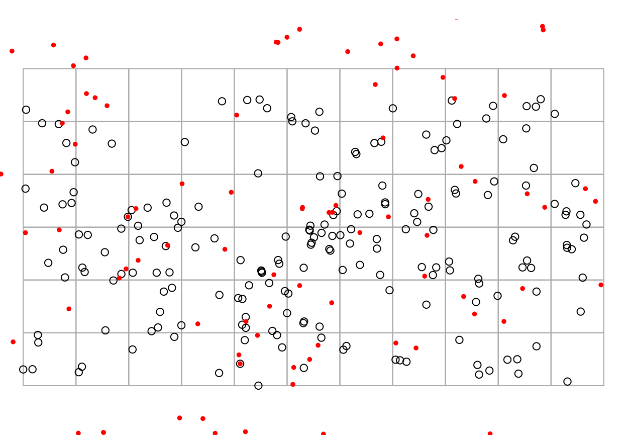
Step 1 - Create an odm-object
All functions with the suffix create_ work with an odm-object which is of type list and contains a numeric matrix for distance and duration as well as the input data that was used to calculate the matrices. The sources are a sf of geometry type POINT and the targets a data.frame.
To make full use of all package functions the sources and targets need to follow at least the following data structures. Additional columns with further attributes can be included in the sources and targets if needed. Coordinates need to be supplied in EPSG:4326.
| source_id | x | y | geom |
|---|---|---|---|
| 1 | 6.977482 | 51.42968 | POINT (6.977482 51.42968) |
| 2 | 6.990986 | 51.43171 | POINT (6.990986 51.43171) |
| 3 | 7.037876 | 51.45258 | POINT (7.037876 51.45258) |
| 4 | 6.978143 | 51.44346 | POINT (6.978143 51.44346) |
| 5 | 7.050361 | 51.44739 | POINT (7.050361 51.44739) |
| target_id | name | category | x | y |
|---|---|---|---|---|
| 1 | amenity_1 | A | 7.02393 | 51.45057 |
| 2 | amenity_2 | B | 6.98052 | 51.41443 |
| 3 | amenity_3 | C | 7.00386 | 51.45200 |
| 4 | amenity_4 | A | 7.00992 | 51.46822 |
| 5 | amenity_5 | B | 6.98880 | 51.43774 |
Execute calculaton
An odm-object can be created sequentially by using
options(openrouteservice.url = "PUT YOUR URL HERE")
odm_result <- calc_odm(profile_string = "foot-walking",
                       source_locations = testdata$od_result$sources,
                       target_locations = testdata$od_result$targets,
                       max_chunk_size = 200)
or in parallel by using
handlers(global = TRUE)
handlers("progress")
registerDoFuture()
plan(multisession, gc = TRUE)
res <- calc_odm_multicore(profile_string = "foot-walking",
                          sources = sources,
                          targets = targets,
                          max_chunk_size = 200,
                          ors_url = "PUT YOUR URL HERE")
Step 2 - Calculate accessibility indicators
Once you have created a odm-list-object calculating indicators is straight forward. The following functions are provided:
| function | arguments | short description | output |
|---|---|---|---|
create_time_distance_sf() |
odm-object |
Calculates distance in meters and duration in minutes from all source points to the closest target location |
sf geometry type POINT
|
create_time_distance_n_sf() |
odm-object, n |
Calculates distance in meters and duration in minutes from all source points to n closest target locations |
sf geometry type POINT
|
create_time_distance_by_cat_sf() |
odm-object, filter_attribute, filter_value |
Calculates distance in meters and duration in minutes from all source points to the closest target location of a chosen category |
sf geometry type POINT
|
create_time_distance_n_by_cat_sf() |
odm-object, filter_attribute, filter_value, n |
Calculates distance in meters and duration in minutes from all source points to n closest target locations of a chosen category |
sf geometry type POINT
|
create_cumulative_sf() |
odm-object, filter_value_type, accessibility_filter_value, search_direction |
All locations which are accessible within the applied time or distance threshold are counted. The count can be calculated in either direction (source to target or target to source) |
sf geometry type POINT
|
create_cumulative_by_cat_sf() |
odm-object, filter_value_type, accessibility_filter_value, search_direction, filter_attribute, filter_value |
All locations which belong to a chosen category and are accessible within the applied time or distance threshold are counted. The count can be calculated in both directions (source to target or target to source) |
sf geometry type POINT
|
create_potential_sf() |
odm-object, filter_value_type, accessibility_filter_value, search_direction, ors_profile |
A decay function is applied to all locations which are accessible within the defined time or distance threshold. The function models a location potential respecting the spatial distribution. Thus, closer features result in higher values. It can be calculated in either direction (source to target or target to source) |
sf geometry type POINT
|
create_potential_by_cat_sf() |
odm-object, filter_value_type, accessibility_filter_value, search_direction, ors_profile, filter_attribute, filter_value |
A decay function is applied to all locations which belong to a chosen category and are accessible within the defined time or distance threshold. The function models a location potential respecting the spatial distribution. Thus, closer features result in higher values. It can be calculated in either direction (source to target or target to source) |
sf geometry type POINT
|
The following example shows the calculation of the distance and duration to the nearest target location using the provided dataset:
result <- create_time_distance_sf(testdata$od_result)
par(mar = c(0,0,1,0))
# Min_Dist could be switched to Min_Time
plot(result["Min_Dist"], key.pos = 1)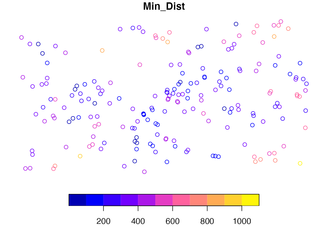
This is only the most basic example but the other listed functions work in a similar way. You just need to add further function parameters.
Step 3 - Aggregate an indicator to an area of interest
Once you have calculated one or more accessibility indicators you might want to aggregate those to statistical spatial units or regular grids. For this use case corresponding aggregation functions are provided:
| function | arguments | short description | output |
|---|---|---|---|
aggregate_expenses() |
aoi_sf, pnt_sf, id_col, crs | Aggregate the sf (geometry type POINT) attributes Min_Dist and Min_Time to an area of interest |
sf geometry type POINT
|
aggregate_accumulation() |
aoi_sf, pnt_sf, id_col, crs | Aggregate the sf (geometry type POINT) attribute MeanCnt or MedianCnt to an area of interest |
sf geometry type POINT
|
aggregate_potential() |
aoi_sf, pnt_sf, id_col, crs | Aggregate the sf (geometry type POINT) attributes MeanPot and MedianPot to an area of interest |
sf geometry type POINT
|
aggregate_coverage_rate_by_threshold() |
aoi_sf, pnt_sf, id_col, crs | Calculate an average coverage rate within an area of interest by applying a threshold filter to one of the sf (geometry type POINT) attributes Min_Dist or Min_Time. A source location is defined as covered if a target location is accessible within the threshold distance or time. |
sf geometry type POINT
|
The following example shows the aggregation and visualization of the minimum distance and duration values calculated in step 2:
library(dplyr)
min_dist_time_sf <- create_time_distance_sf(testdata$od_result) %>%
  sf::st_transform(4647)
# Add targets for plotting
targets_sf <- sf::st_as_sf(testdata$od_result$targets, coords = c("x", "y")) %>%
  sf::st_set_crs(4326) %>%
  sf::st_transform(4647)
result_sf <- aggregate_expenses(aoi_sf = testdata$grid_500m,
                                pnt_sf = min_dist_time_sf,
                                id_col = "id",
                                crs = 4647)
par(mar = c(0,0,1,0))
# MedianDist could be switched to MedianTime
plot(result_sf["MedianDist"], border = "darkgrey", key.pos = 1, reset = FALSE)
plot(min_dist_time_sf$geom, pch = 20, cex = 1, add = TRUE)
plot(targets_sf$geometry, col = "red", pch = 20, cex = .8, add = TRUE)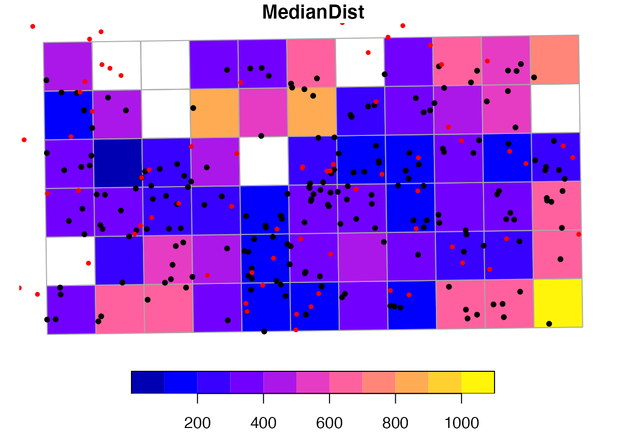
This is only one example but the other listed functions work in a similar way. You just need to provide the respective accessibility indicator result to the aggregation function.
Step 4 - Merge multiple aggregated indicator results (optional)
For convenience a merge function is provided which allows you to easily combine the sf objects of multiple aggregated indicators which have been aggregated to the same areas of interest.
# Travel expenses
min_dist_time_sf <- create_time_distance_sf(testdata$od_result)
expenses_sf <- aggregate_expenses(aoi_sf = testdata$grid_500m,
                                  pnt_sf = min_dist_time_sf,
                                  id_col = "id",
                                  crs = 4647)
# Accumulation
cnt_sf <- create_cumulative_sf(odm_object = testdata$od_result,
                               filter_value_type = "distance",
                               accessibility_filter_value = 750,
                               search_direction = "to_target")
cumulative_sf <- aggregate_accumulation(aoi_sf = testdata$grid_500m,
                                        pnt_sf = cnt_sf,
                                        id_col = "id",
                                        crs = 4647)
# Potential
pot_sf <- create_potential_sf(odm_object = testdata$od_result,
                              filter_value_type = "distance",
                              accessibility_filter_value = 750,
                              search_direction = "to_target",
                              ors_profile = "foot-walking")
potential_sf <- aggregate_potential(aoi_sf = testdata$grid_500m,
                                    pnt_sf = pot_sf,
                                    id_col = "id",
                                    crs = 4647)
# Coverage rate in %
coverage_sf <- aggregate_coverage_rate_by_threshold(aoi_sf = testdata$grid_500m,
                                                    pnt_sf = min_dist_time_sf,
                                                    id_col = "id",
                                                    threshold_col = "Min_Dist",
                                                    threshold_value = 350,
                                                    crs = 4647)
# Merge
merged_sf <- merge_indicators(aoi_sf = testdata$grid_500m, id_col = "id",
                              expenses_sf, cumulative_sf, potential_sf,
                              coverage_sf)
# Remove the the geometry column just for table presentation
knitr::kable(head(sf::st_drop_geometry(merged_sf), 5))| id | MedianDist | MedianTime | MeanCnt | MedianCnt | MeanPot | MedianPot | Mean_CoverageRate |
|---|---|---|---|---|---|---|---|
| 1 | 383.160 | 4.597750 | 2.5 | 2.5 | 218.80910 | 218.20230 | 25 |
| 2 | 698.425 | 8.380833 | 1.0 | 1.0 | 75.13072 | 75.13072 | 0 |
| 3 | 607.235 | 7.286667 | 0.5 | 0.5 | 50.00000 | 50.00000 | 50 |
| 4 | 334.500 | 4.013833 | 8.0 | 8.0 | 683.06632 | 683.06632 | 100 |
| 5 | 198.420 | 2.380833 | 7.8 | 7.0 | 714.32792 | 647.56115 | 80 |
This last example gives a concluding first impression of the functions provided within package. See ?odmind for more details!